Deep Reinforcement Learning: how to teach spiders to walk

On today’s episode of “how to teach machines to do things every living creature is capable of” I will show you how to make a little spider-robot walk. In a nutshell, we will discuss how to build black box algorithm that takes in robot architecture and produces control policy for this robot such that it will be able to run as fast as possible.

The main component of the solution is an algorithm called Advantage Actor Critic (A2C) with Advantage estimate via Generalized Advantage Estimation (GAE).

The following contains math, TensorFlow implementation and plenty of demos of running gaits agents converged to. Let’s dive deep into Reinforcement Learning!

All the code for this article can be found in this repository.

Table of content:

– Task
– Why Reinforcement Learning?
– Reinforcement Learning formulation
– Policy gradient
– Diagonal Gaussian Policies
– Variance reduction by introducing the Critic
– Pitfalls
– Summary

Task

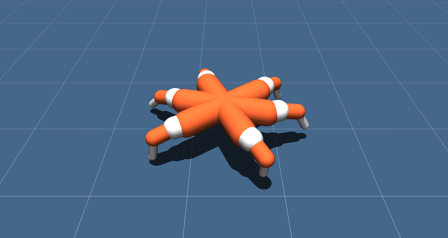
We are going to use MuJoCo simulation for our purposes of building and teaching the robot. We will skip the step of creating a model of the spider and Python interface to simulation, because that is not that fun and pretty straight forward 🙂 If you are having trouble on this step check out demos that go along with MuJoCo itself or source code of MuJoCo-environments in Gym OpenAI. Also the model of the spider from this article can be found in the repository.

The agent will receive lots of numbers from MuJoCo: relative poses, angles, velocities, accelerations of robot’s body parts, e.t.c. Summing up to ~800 features. Let’s go full Deep Learning approach, we will not deepen into figuring out what they really mean under the hood of the physics engine. The main thing is that they will be sufficient for the agent to somewhat fully recover and understand what is going on around it.

The output will be 18 real numbers which is the number of degrees of freedom. They represent angles of hinges on which robot’s limbs rotate.

Finally, the goal of the agent will be to maximize total reward over an episode. We will stop the episode if the robot falls or a certain amount of steps passes. In our case it is 3000 steps or 15 seconds. The agent will receive a reward on every step calculated by the next formula:

To put it another way, the agent’s goal will be to increase its coordinate and not to fall until the end of an episode.

Our ultimate goal is to find a function which will allow the agent to obtain the most reward over an episode. Sounds challenging, does not it? 🙂 Let’s see how Deep Reinforcement Learning pulls it off.

Why Reinforcement Learning?

Present approaches to similar tasks of making legged robots walk include classical practices in robotics studied in optimal control and trajectory optimization: LQR, QP, convex optimization. See paper by Boston Dynamics about Atlas robot.

These techniques are somewhat “hard-code” as they demand introducing a lot of concrete details and domain knowledge into the algorithm. They do not have any learning parts, optimization occurs in-place.

On the other hand, Reinforcement Learning (further RL) does not require injecting domain knowledge into the algorithm leading to more general, robust and scalable solutions.

Reinforcement Learning formulation

In RL problem we take agent-environment interaction as a sequence of pairs (state, reward) and transitions between them – actions.

Notion definition:

• – policy, strategy by which agent chooses action given state, it is a conditional probability,
• – action is a random value from distribution with fixed ,
• – trajectory or rollout, sequence of consecutive states agent visited .

Note: we could have treated policy as a function , but we want agent’s actions to be stochastic which in turn facilitates exploration. That is we take actions slightly different from which agent chooses. Therefore mathematical tools are slightly more complicated.

The goal of the agent is to maximize expected return:

Finally, we can formulate RL objective, to find:

where – optimal policy.

See more details here: OpenAI Spinning Up.

Policy gradient

It is remarkable that rigorous formulation of the RL as optimization problem allows us to use optimization tools studied for a long time. One of which is gradient descent. Just imagine how it would be cool if we could take gradient of expected return over model parameters: . In this case, the weights update rule would be just:

As it turns out, that is exactly the idea behind policy gradient. Rigorous proof of it is beyond the scope of this article. You can check it out here. The gradient looks as follows:

Therefore the loss for our model is:

Quick note, , and – is the output of our model at the moment agent was in the state . The minus comes from the fact that we would like to maximize . During the training process we will calculate the gradients on batches of steps and sum them up in order to reduce variance (noise in the data originating from stochasticity of the environment).

This is an already working algorithm called REINFORCE. It can find solutions for simple problems, such as the “CartPole-v1” environment.

Let’s go through the agent’s code:

class ActorNetworkDiscrete:
    def __init__(self):
        self.state_ph = tf.placeholder(tf.float32, shape=[None, observation_space])
        l1 = tf.layers.dense(self.state_ph, units=20, activation=tf.nn.relu)
        output_linear = tf.layers.dense(l1, units=action_space)

        output = tf.nn.softmax(output_linear)
        self.action_op = tf.squeeze(tf.multinomial(logits=output_linear,num_samples=1), 
                                    axis=1)

        # Training
        output_log = tf.nn.log_softmax(output_linear)

        self.weight_ph = tf.placeholder(shape=[None], dtype=tf.float32)
        self.action_ph = tf.placeholder(shape=[None], dtype=tf.int32)

        action_one_hot = tf.one_hot(self.action_ph, action_space)
        responsible_output_log = tf.reduce_sum(output_log * action_one_hot, axis=1)
        self.loss = -tf.reduce_mean(responsible_output_log * self.weight_ph)

        optimizer = tf.train.AdamOptimizer(learning_rate=actor_learning_rate)
        self.update_op = optimizer.minimize(self.loss)

actor = ActorNetworkDiscrete()

We have got a little perceptron of this architecture: (observation_space, 10, action_space)[for CartPole it is (4, 10, 2)]. tf.multinomial serves us the purpose of picking actions randomly weighted by output of the neural network. To acquire agent’s will we will call:

action = sess.run(actor.action_op, 
                  feed_dict={actor.state_ph: observation})

Training loop looks as follows:

batch_generator = generate_batch(environments,
                                 batch_size=batch_size)

for epoch in tqdm_notebook(range(epochs_number)):
    batch = next(batch_generator)

    # Reminder: batch item consists of [state, action, total reward]
    # Train actor
    _, actor_loss = sess.run([actor.update_op, actor.loss], 
                             feed_dict={actor.state_ph: batch[:, 0],
                                        actor.action_ph: batch[:, 1],
                                        actor.weight_ph: batch[:, 2]})

Batch generator runs agent in the environment and collects training data. Batch consists of such tuples: .

The task of writing a good batch generator is on its own a little challenging. The main challenge is that neural network inference (sess.run()) is expensive compared to one step of the simulation (even MuJoCo). For the sake of boosting we can exploit the fact that neural networks can be run on batches of data with little overhead. We will use many parallel environments. Even if we run them in sequence it will significantly boost training compared to a single environment.

# Vectorized environments with gym-like interface
from baselines.common.vec_env.subproc_vec_env import SubprocVecEnv
from baselines.common.vec_env.dummy_vec_env import DummyVecEnv

def make_env(env_id, seed):
    def _f():
        env = gym.make(env_name)
        env.reset()

        # Desync environments
        for i in range(int(200 * seed // environments_count)):
            env.step(env.action_space.sample())
        return env
    return _f

envs = [make_env(env_name, seed) for seed in range(environments_count)]

# Can be switched to SubprocVecEnv to parallelize on cores 
# (for computationally heavy envs)
envs = DummyVecEnv(envs)


# Source: 
# https://github.com/openai/spinningup/blob/master/spinup/algos/ppo/core.py
def discount_cumsum(x, coef):
    """
    magic from rllab for computing discounted cumulative sums of vectors.
    input: 
        vector x, 
        [x0, 
         x1, 
         x2]
    output:
        [x0 + discount * x1 + discount^2 * x2,  
         x1 + discount * x2,
         x2]
    """
    return scipy.signal.lfilter([1], [1, float(-coef)], x[::-1], axis=0)[::-1]


def generate_batch(envs, batch_size, replay_buffer_size):
    envs_number = envs.num_envs
    observations = [[0 for i in range(observation_space)] for i in range(envs_number)]
    
    # [state, action, discounted reward-to-go]
    replay_buffer = np.empty((0,3), np.float32)
    
    # [state, action, reward] rollout lists for every environment instance
    rollouts = [np.empty((0, 3)) for i in range(envs_number)]

    while True:
        history = {'reward': [], 'max_action': []}
        replay_buffer = replay_buffer[batch_size:]
        
        # Main sampling cycle
        while len(replay_buffer) < replay_buffer_size:
            # Here policy acts in environments. Note that it chooses actions for all
            # environments in one batch, therefore expensive sess.run is called once.
            actions = sess.run(actor.action_op, 
                               feed_dict={actor.state_ph: observations})
            observations_old = observations
            observations, rewards, dones, _ = envs.step(actions)
            
            history['max_action'].append(np.abs(actions).max())
            
            time_point = np.array(list(zip(observations_old, actions, rewards)))
            for i in range(envs_number):
                # Regular python-like append
                rollouts[i] = np.append(rollouts[i], [time_point[i]], axis=0) 
            
            # Process done==True environments
            if dones.all():
                print('WARNING: envs are in sync!! This makes sampling inefficient!')

            done_indexes = np.arange(envs_number)[dones]
            for i in done_indexes:
                rewards_trajectory = rollouts[i][:, 2].copy()
                history['reward'].append(rewards_trajectory.sum())

                rollouts[i][:, 2] = discount_cumsum(rewards_trajectory,
                                                    coef=discount_factor)
                replay_buffer = np.append(replay_buffer, rollouts[i], axis=0)
                rollouts[i] = np.empty((0, 3))
        
        # Shuffle before yield to become closer to i.i.d.
        np.random.shuffle(replay_buffer)
        
        # Truncate replay_buffer to get the most relevant feedback from environment
        replay_buffer = replay_buffer[:replay_buffer_size]
        yield replay_buffer[:batch_size], history

# Make a test yield
a = generate_batch(envs, 8, 64)
# Makes them of equal lenght
for i in range(10):
    next(a)
next(a)[0]

Acquired agent can play in environments with finite actions space. (e.g. Atari). This output format does not fit our task. The agent controlling the robot must output vector from , where – number of degrees of freedom.

Note: you can formulate your robot control task in a way that action space is finite. One can divide the continuum of activations into bins and make agent pick bins instead of vectors as done here.) Though this approach may introduce action space sparsity problems.

Diagonal Gaussian Policies

The method of Diagonal Gaussian Policies is to shape model output so that it will output parameters of n-dimensional normal distribution in which it thinks the correct action resides. To be more specific, parameters are – expected value and – standard deviation. As the agent needs to act we will ask these numbers and sample random value from the corresponding distribution. This way we made our model output vector from and made it stochastic. The most important part is that by fixing a class of the output distribution we made possible for us to us to calculate and, hence, policy gradient.

Note: we can fix as hyperparameter, thereby reducing output dimensionality. Practice shows that it does not hurt that much, but on the contrary, stabilises training.

More on stochastic policies.

New agent’s code:

epsilon = 1e-8

def gaussian_loglikelihood(x, mu, log_std):
    pre_sum = -0.5 * (((x - mu) / (tf.exp(log_std) + epsilon))**2 \ 
        + 2 * log_std + np.log(2 * np.pi))
    return tf.reduce_sum(pre_sum, axis=1)

class ActorNetworkContinuous:
    def __init__(self):
        self.state_ph = tf.placeholder(tf.float32, shape=[None, observation_space])

        l1 = tf.layers.dense(self.state_ph, units=100, activation=tf.nn.tanh)
        l2 = tf.layers.dense(l1, units=50, activation=tf.nn.tanh)
        l3 = tf.layers.dense(l2, units=25, activation=tf.nn.tanh)
        mu = tf.layers.dense(l3, units=action_space)

        log_std = tf.get_variable(name='log_std', 
                                  initializer=-0.5 * np.ones(action_space,  
                                                             dtype=np.float32))
        std = tf.exp(log_std)

        self.action_op = mu + tf.random.normal(shape=tf.shape(mu)) * std

        # Training
        self.weight_ph = tf.placeholder(shape=[None], dtype=tf.float32)
        self.action_ph = tf.placeholder(shape=[None, action_space], dtype=tf.float32)

        action_logprob = gaussian_loglikelihood(self.action_ph, mu, log_std)
        self.loss = -tf.reduce_mean(action_logprob * self.weight_ph)
        
        optimizer = tf.train.AdamOptimizer(learning_rate=actor_learning_rate)
        self.update_op = optimizer.minimize(self.loss)

Training loop stays the same.

Finally, we can test REINFORCE on our task. Hereinafter the goal of the agent is to move to the right.

Slow and steady crawls to its goal.

Reward-to-go

Let’s notice that our gradient contains redundant terms. For every step we weight the gradient of the logarithm by the sum of the rewards over the entire trajectory. Thus, judging an agent’s actions by its achievements from the past. Common sense suggests there is something wrong with this. It turns out leaving out these extra terms makes training more stable. Therefore our gradient

transforms to this

Find 10 differences 🙂

While math is okay with these extra terms they increase variance in our data. Now the agent will focus only on the rewards it got after the specific action.

Due to this improvement the mean reward increased. One of the obtained agents learned to use its forelimbs to achieve the goal:

Variance reduction by introducing the Critic

The essence of the following improvements is to reduce variance coming from stochastic nature of the transitions between states of the environment.

We will introduce a model that will predict expected sum of the rewards received by the agent from state till the end of the trajectory, i.e. Value-function.

Value-function predicts expected return, given that our policy starts the game from a specific state. Same with Q-function, but the first action is also fixed.

Introducing the Critic

This is how the gradient looks like when we use reward-to-go:

Notice that the coefficient by the gradient of the logarithm is nothing else, but a sample from the Value-function.

We weight the gradient of the logarithm with one sample from the specific trajectory which is not right. We can approximate Value-function with some model, for example, a neural network and ask it to predict required values, reducing variance even more. We will call this model Critic and will teach it simultaneous with policy. Therefore, the formula of the gradient can be written as follows:

We decreased variance, but at the same time we introduced bias into our algorithm, as neural networks can make approximation mistakes (as every other approximation algorithm does). Tradeoff turns out to be good in this case. In machine learning such situations are called bias-variance tradeoff.

Critic will fit Value-function by regression on samples of reward-to-go, collected in the environment. We will take MSE as a loss function. That is loss is:

The code of the critic:

class CriticNetwork:
    def __init__(self):
        self.state_ph = tf.placeholder(tf.float32, shape=[None, observation_space])

        l1 = tf.layers.dense(self.state_ph, units=100, activation=tf.nn.tanh)        
        l2 = tf.layers.dense(l1, units=50, activation=tf.nn.tanh)
        l3 = tf.layers.dense(l2, units=25, activation=tf.nn.tanh)
        output = tf.layers.dense(l3, units=1)
        
        self.value_op = tf.squeeze(output, axis=-1)

        # Training
        self.value_ph = tf.placeholder(shape=[None], dtype=tf.float32)
        
        self.loss = tf.losses.mean_squared_error(self.value_ph, self.value_op)
        
        optimizer = tf.train.AdamOptimizer(learning_rate=critic_learning_rate)
        self.update_op = optimizer.minimize(self.loss)

Training loop becomes:

batch_generator = generate_batch(envs,
                                 batch_size=batch_size)

for epoch in tqdm_notebook(range(epochs_number)):
    batch = next(batch_generator)

    # Reminder: batch item consists of [state, action, value, reward-to-go]
    # Train actor
    _, actor_loss = sess.run([actor.update_op, actor.loss], 
                             feed_dict={actor.state_ph: batch[:, 0],
                                        actor.action_ph: batch[:, 1],
                                        actor.weight_ph: batch[:, 2]})
    
    # Train critic
    for j in range(10):
        _, critic_loss = sess.run([critic.update_op, critic.loss], 
                                  feed_dict={critic.state_ph: batch[:, 0],
                                             critic.value_ph: batch[:, 3]})

Now batches contain another one number, Value calculated by the Critic in batch generator.
i.e. batch format is .

Nothing stops us from training the Critic till convergence inside the loop. So we will make several gradient descent steps, thus, improving approximation of the Value-function and reducing bias. However, this approach requires large batch size to avoid overfitting. The similar statement about training policy is wrong. It has to have instant feedback from the environment for training, otherwise we may find ourselves punishing policy for decisions it would not already make. Algorithms with this property are called on-policy.

Baselines in Policy Gradients

It is possible to derive that we can substitute Value-function with any representative of a special class of the functions in our gradient formula. This function can be dependent on . These functions are called baselines. (Derivation of this fact) These functions seem to be profitable as baselines:

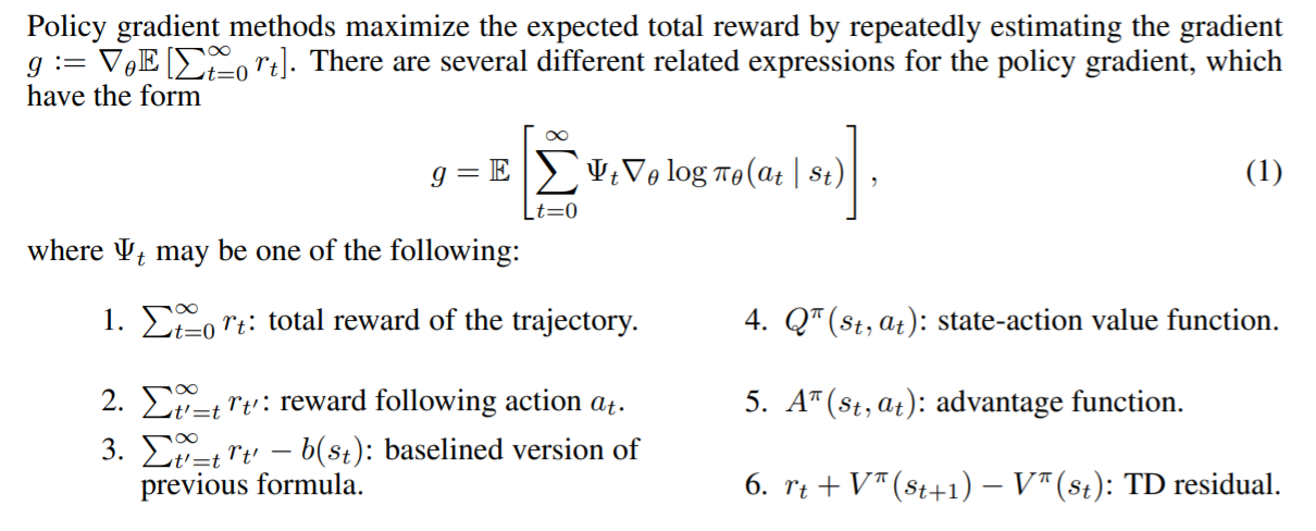
Source: GAE paper.

Different baselines give different results depending on the task. Advantage-function gives the most profit in our task.

There is a little intuition behind it. When we use Advantage-function we let the agent assess its actions by itself. As agent learns in the environment, its standards are getting higher. Its past experience serves as a reference level for the agent. The ideal agent will be good at the game and will evaluate its actions as having Advantage equal to 0 and, thus, gradient equal to 0.

Advantage estimation with Value-function

A little reminder of the definition of Advantage:

It is not clear how to approximate this function explicitly. A trick will come to the rescue: we can reduce calculation of Advantage-function to calculation of Value-function.

Let’s define – Temporal Difference residual (TD-residual). It is not hard to prove that this function approximates Advantage:

And now instead of an estimate of Value-function we will pass Advantage estimate into policy training. Few lines of code will do the trick.

Acquired algorithm is called Advantage Actor-Critic.

def estimate_advantage(states, rewards):
    values = sess.run(critic.value_op, feed_dict={critic.state_ph: states})
    deltas = rewards - values
    deltas = deltas + np.append(values[1:], np.array([0]))
    
    return deltas, values

Generated agents demonstrate the ability to confidently walk and usage of all the limbs in sync:

Generalized Advantage Estimation

Somewhat recent paper (2015) “High-dimensional continuous control using generalized advantage estimation” suggests using more effective Advantage estimation with Value-function. It reduces variance even more:

where:

• – TD-residual,
• – discount-factor (hyperparameter),
• – hyperparameter.

This approach can be interpreted as special task-agnostic reward shaping. Full interpretation can be found in the paper itself.

Implementation:

def discount_cumsum(x, coef):
    # Source: 
    # https://github.com/openai/spinningup/blob/master/spinup/algos/ppo/core.py
    """
    magic from rllab for computing discounted cumulative sums of vectors.
    input: 
        vector x, 
        [x0, 
         x1, 
         x2]
    output:
        [x0 + discount * x1 + discount^2 * x2,  
         x1 + discount * x2,
         x2]
    """
    return scipy.signal.lfilter([1], [1, float(-coef)], x[::-1], axis=0)[::-1]


def estimate_advantage(states, rewards):
    values = sess.run(critic.value_op, feed_dict={critic.state_ph: states})
    deltas = rewards - values
    deltas = deltas + discount_factor * np.append(values[1:], np.array([0]))
    
    advantage = discount_cumsum(deltas, coef=lambda_factor * discount_factor)
    return advantage, values

When the algorithm used too little batch size, it converged to some local minima, which are quite entertaining to observe. Here agent uses one of its limbs as cane and pushes itself with the others:

Here the agent did not converge to using jumps and just walks fast. Also notice how it behaves when stumbles – turns around and continues running:

The best agent, it is him on the top of the article. It moves by hopping around and all limbs are up in the air during every hop. The developed ability to balance lets the agent correct its trajectory on the fly if mistake occurs:

Pitfalls

Machine learning is known for its dimensionality of error space. Any error and you get a completely unable algorithm. RL takes this problem to a whole new level.

Source

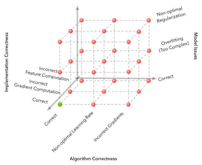
Here we describe some difficulties which occured on the way of development.

1. Algorithm is surprisingly sensitive to hyperparameters. Algorithm was observed to gain massive quality from little changes in learning rate. Change from 3e-4 to 1e-4 drastically increased the agent’s final score.
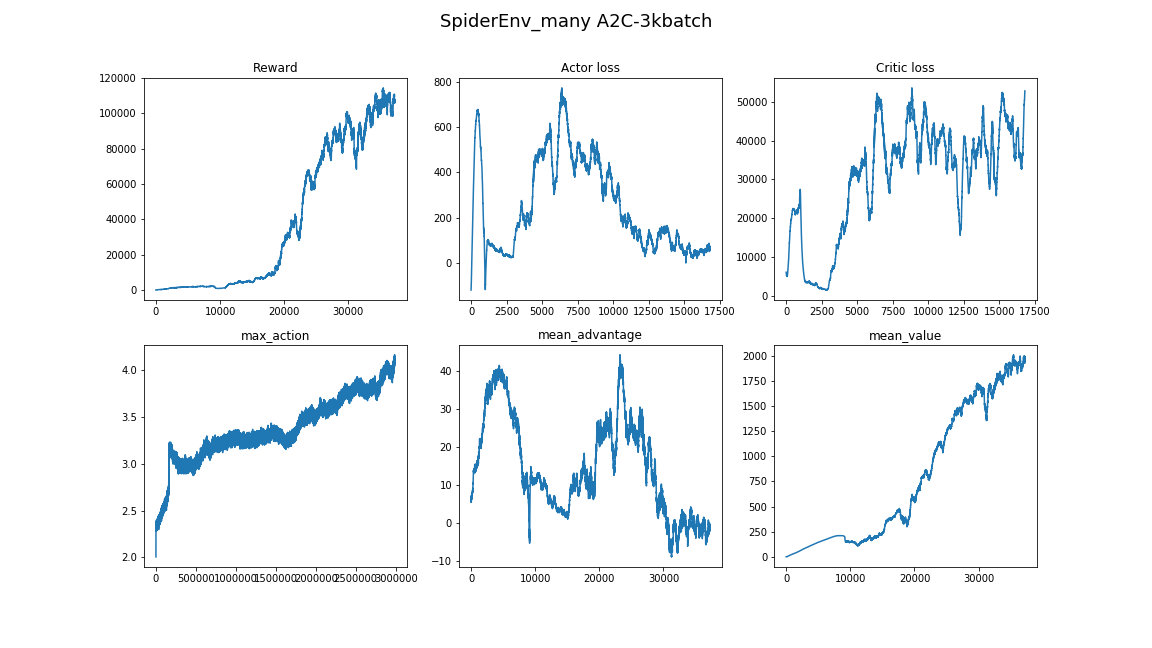
2. The size of the batch is completely different from those in other fields of Deep Learning. It is common to use 32-256 batch size in image classification. But here it is better to have your batch size on the order of several thousands. In our case 3000 works fine. 
3. The training process varies from launch to launch. It is better to run experiments several times. Sometimes random seeds are unlucky.
4. Training in such a complex environment takes its time and the progress is not uniform. For example, the best agent trained for 8 hours and it showed results worse than a random baseline for the first 3 hours. Therefore, it is better to start with small toy environments from the Gym.
5. A good way of searching suitable hyperparameters and model architectures is to peep at the papers and implementations of algorithms close to your task. (do not overfit though!) 
   For more info on which parameters work for on-policy algorithms controlling legged robots check out paper “What Matters In On-Policy Reinforcement Learning? A Large-Scale Empirical Study“.

See more nuances about Deep RL in Deep Reinforcement Learning Doesn’t Work Yet.

Conclusion

Acquired algorithm solves the task convincingly. We found the function which controls the robot in an agile and confident manner.

The next logical step is to study descendants of A2C: PPO and TRPO. They are focused on improving sample efficiency of the A2C, i.e. the time it takes an algorithm to converge. Also they are capable of solving more complex tasks. Not so long ago PPO + Automatic Domain Randomization solved Rubik’s cube with a robot hand.

Again, all the code for this article can be found in this repository.

Hope you enjoyed the article and you got inspired by the things Deep Reinforcement Learning is already capable of.

Thanks for your attention!

Useful links:

• Welcome to Spinning Up in Deep RL!
• CS 294: Deep Reinforcement Learning, Fall 2017
• CS 285: Deep Reinforcement Learning, Decision Making and Control
• High-dimensional continuous control using generalized advantage estimation
• OpenAI Baselines: high-quality implementations of reinforcement learning algorithms

Thanks to @pinkotter, @Vambala, @andrey_probochkin, @pollyfom and @suriknik  for the help with the project.
In particular, @Vambala and @andrey_probochkin for creating an excellent MuJoCo environment.